Sentiment Analysis with Embeddings + RNN / GRU / LSTM

This page summarizes how the sentiment classifier was built: data preparation, embedding strategy, training setup, model variants (baseline vs GRU vs LSTM), and the visuals used to validate results. Code is intentionally shown only as small snippets (no full notebook dump).

NLP Sequence Classification Embeddings RNN • GRU • LSTM

Task

Sentiment classification (positive vs negative vs neutral vs irrelevant )

Input

Tokenized text sequences with padding/truncation

Output

Probability score + class label

1) Data & Preprocessing

Text was cleaned and standardized before training. The objective was to reduce noise without losing meaning (especially around negations like “not good”).

Lowercasing + basic normalization
Tokenization → integer sequences
Padding/truncation to a fixed length
Train/validation split with consistent random seed

# Tokenization + padding (snippet)
tokenizer = Tokenizer(num_words=VOCAB_SIZE, oov_token="<OOV>")
tokenizer.fit_on_texts(train_texts)

X_train = pad_sequences(tokenizer.texts_to_sequences(train_texts),
                        maxlen=MAX_LEN, padding="post", truncating="post")
X_val   = pad_sequences(tokenizer.texts_to_sequences(val_texts),
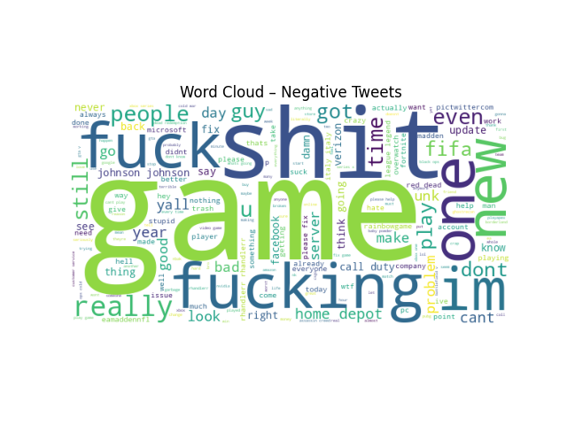
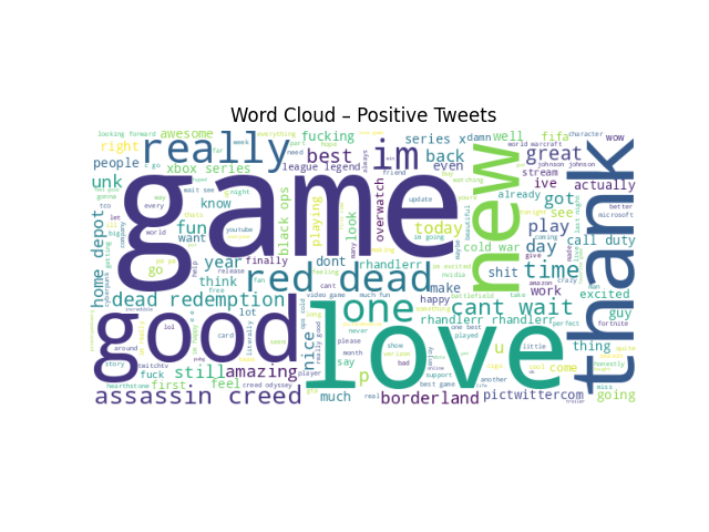
                        maxlen=MAX_LEN, padding="post", truncating="post")

Visual checks used

Word cloud to quickly inspect dominant vocabulary

2) Embedding Strategy

The embedding layer converts word IDs into dense vectors so the model can learn semantic relationships. We used trainable embeddings as the default approach.

Vocab: 20000 (default constant)

Dim: 128 & 68

Len: 163

# Embedding layer (snippet)
model = Sequential([
  Embedding(input_dim=VOCAB_SIZE, output_dim=EMBED_DIM, input_length=MAX_LEN),
  ...

Optional upgrade: use pre-trained embeddings (e.g., GloVe) to improve generalization on small datasets.

Baseline vs Sequence Models

RNN: Embedding → SimpleRNN → dense classifier
GRU: Embedding → GRU → dense classifier
LSTM: Embedding → LSTM → dense classifier

# Baseline (snippet)
Embedding(...)
GlobalAveragePooling1D()
Dense(4, activation="sigmoid")

3) Model Variants Compared

The main comparison was whether sequence-aware units (RNN/GRU/LSTM) improved over an embedding-only baseline. GRU/LSTM typically help when longer dependencies matter and gradients need more stability.

SimpleRNN

Good for fundamentals + quick tests; limited for long context.

Embedding(...)
SimpleRNN(UNITS)
Dense(4, "sigmoid")

GRU

Fewer gates than LSTM; often faster with strong performance.

Embedding(...)
GRU(UNITS)
Dense(4, "sigmoid")

LSTM

Strong for longer sequences; more parameters / compute.

Embedding(...)
LSTM(UNITS)
Dense(4, "sigmoid")

4) Training Setup

Training used a standard binary classification setup.

Loss: binary cross-entropy
Optimizer: Adam
Regularization: dropout (if overfitting appears)
Callbacks: early stopping / checkpoints

# Compile + train (snippet)
model.compile(optimizer="adam",
              loss="binary_crossentropy",
              metrics=["accuracy"])

history = model.fit(X_train, y_train,
                    validation_data=(X_val, y_val),
                    epochs=EPOCHS,
                    batch_size=BATCH_SIZE)

Training curves

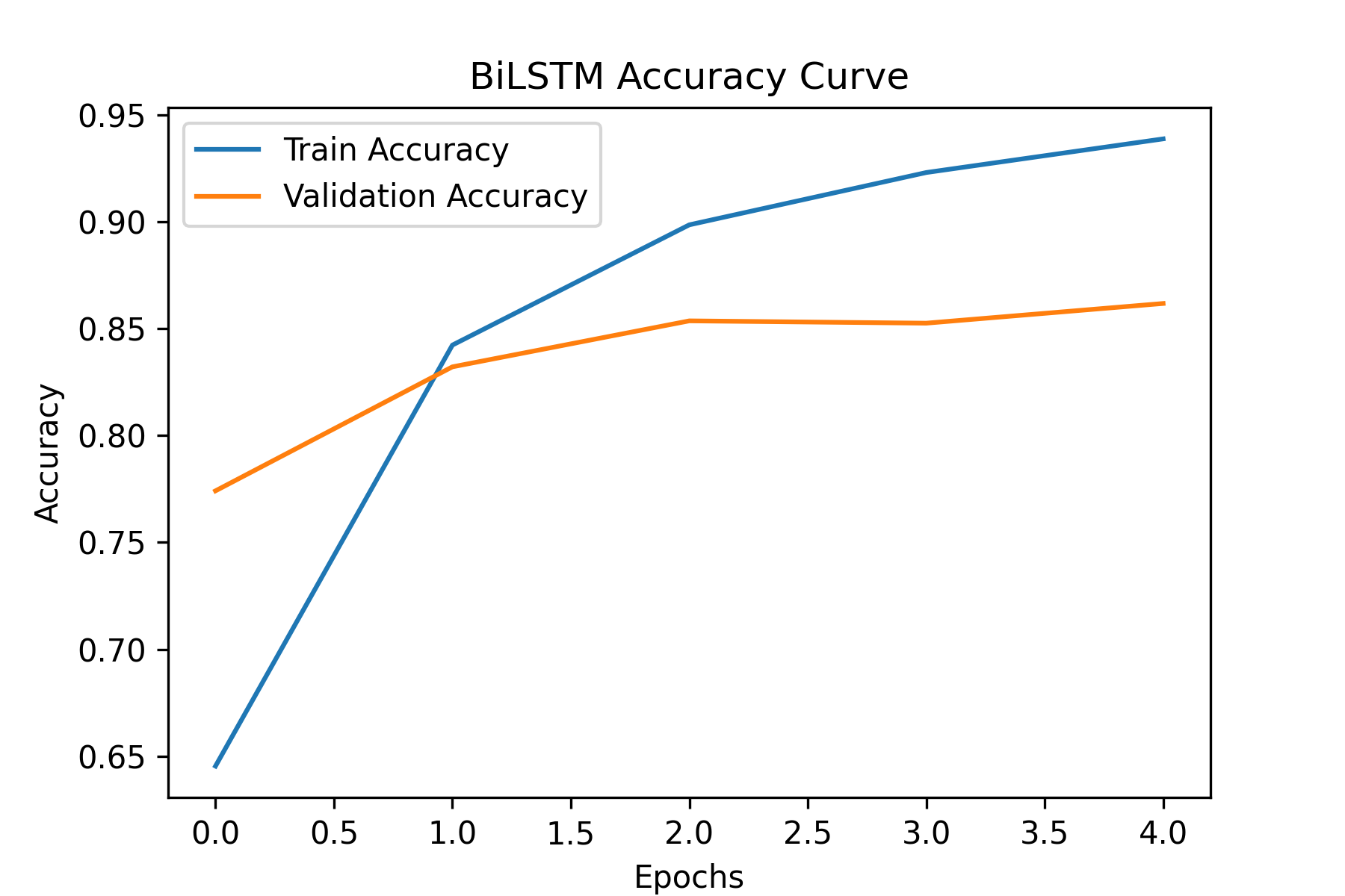
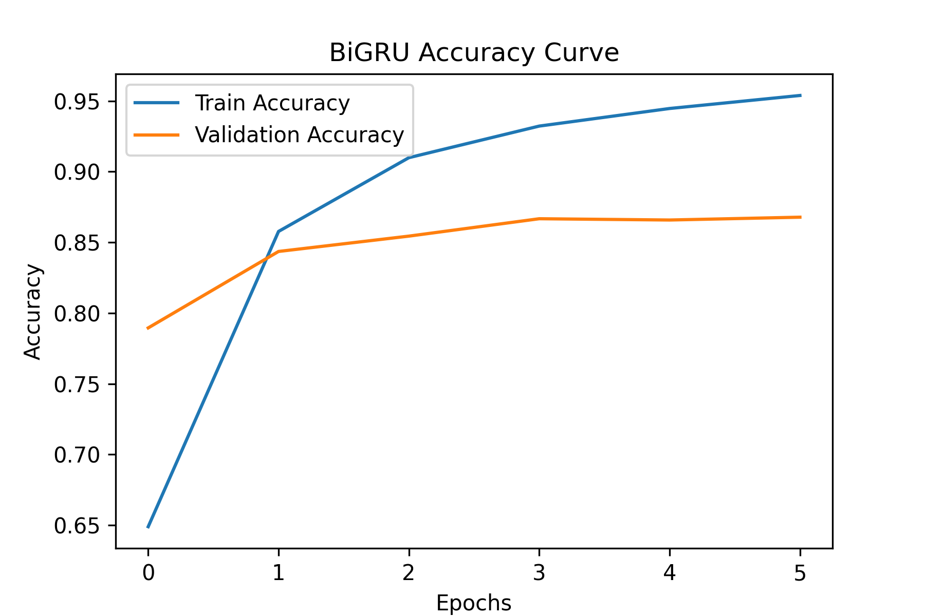
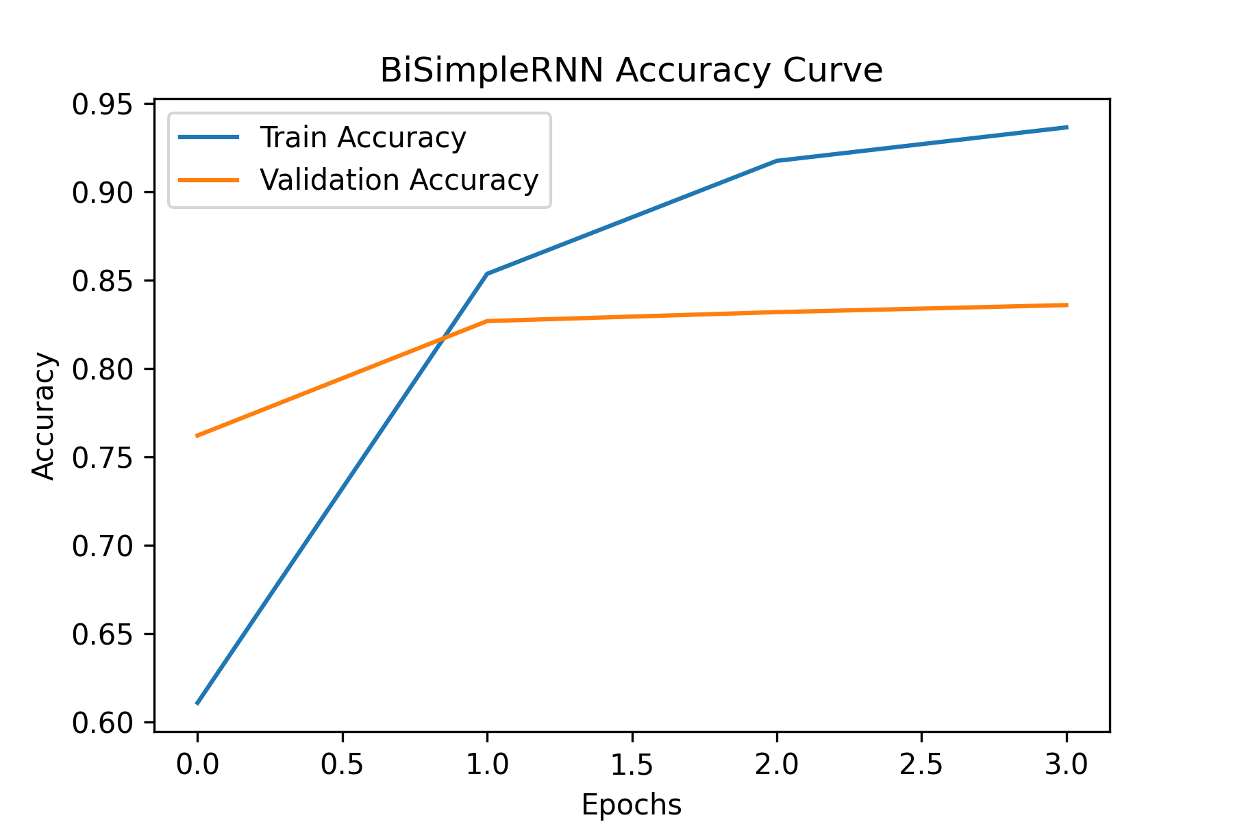
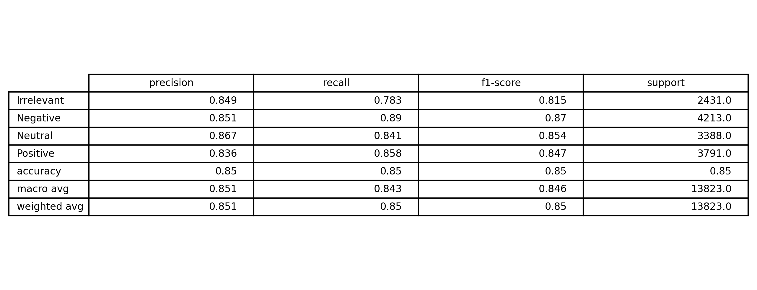
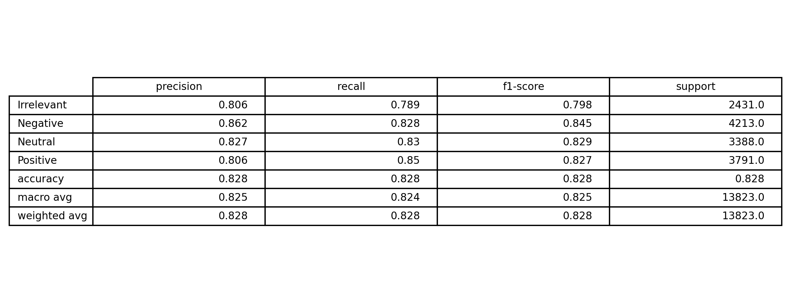
Training/validation curves (placeholder)

5) Evaluation & Results

Evaluation focused on both metrics and error patterns (examples that break the model).

Accuracy, Precision, Recall, F1

y_pred = np.argmax(model_gru.predict(X_test), axis=1)
y_true = np.argmax(y_test, axis=1)
print(classification_report(y_true, y_pred_gru, target_names=le.classes_))